Obtaining Quantum Yield with JOYAI
Step 1: Upload the desired file in the "Modeling" tab.
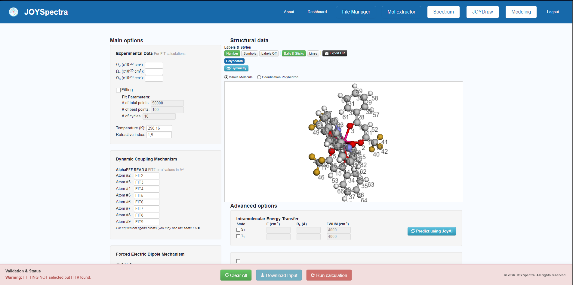
Step 2: In the left panel under "Experimental Data", fill in the values for the intensity parameters (Ω2, Ω4, and Ω6).
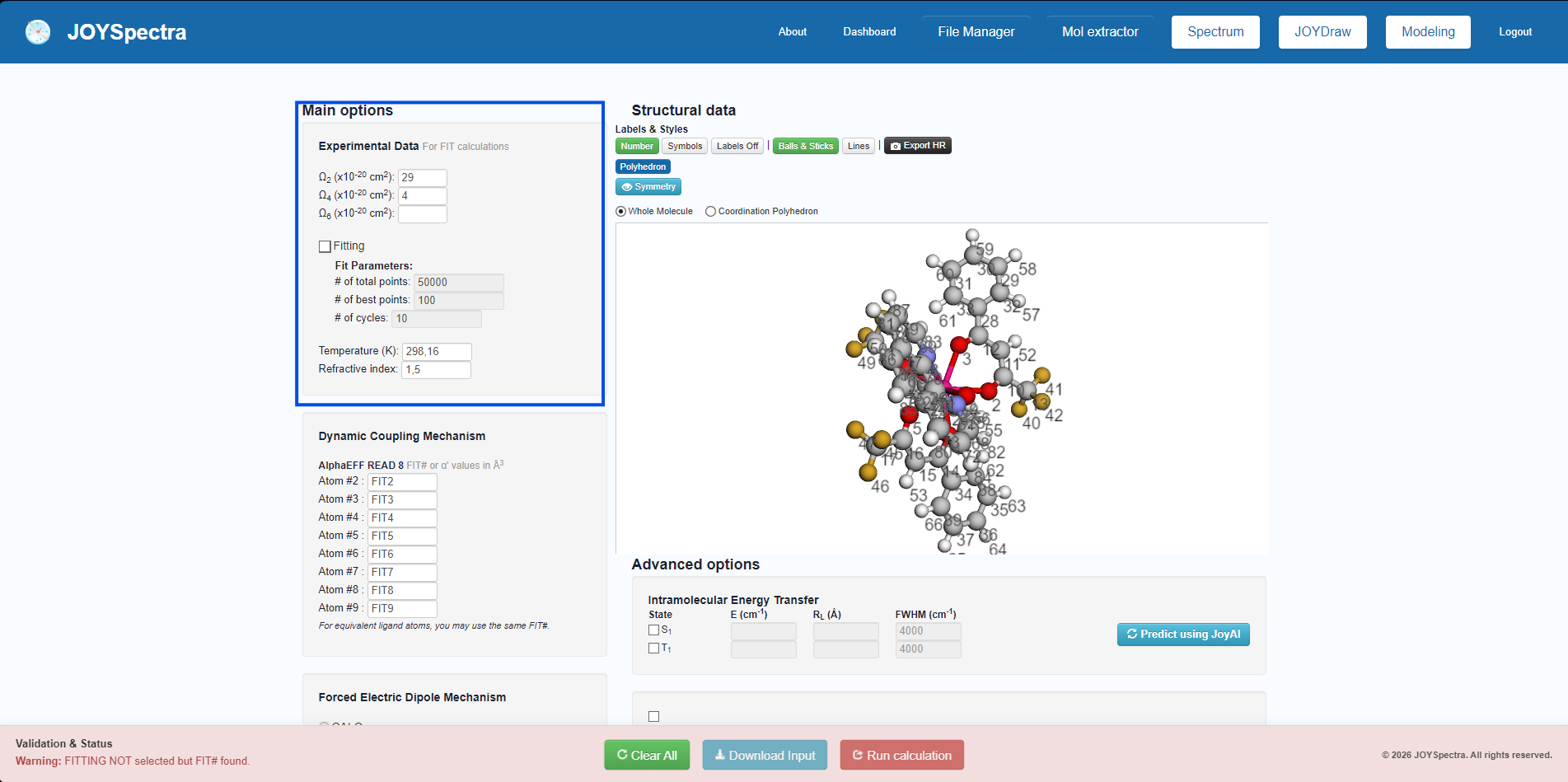
Step 3: In the "Dynamic Coupling Mechanism" and "Forced Electric Dipole Mechanism" sections, assign the corresponding FIT# identifications for each atom, making sure to keep the exact same FIT# numbering in both panels for each listed atom.
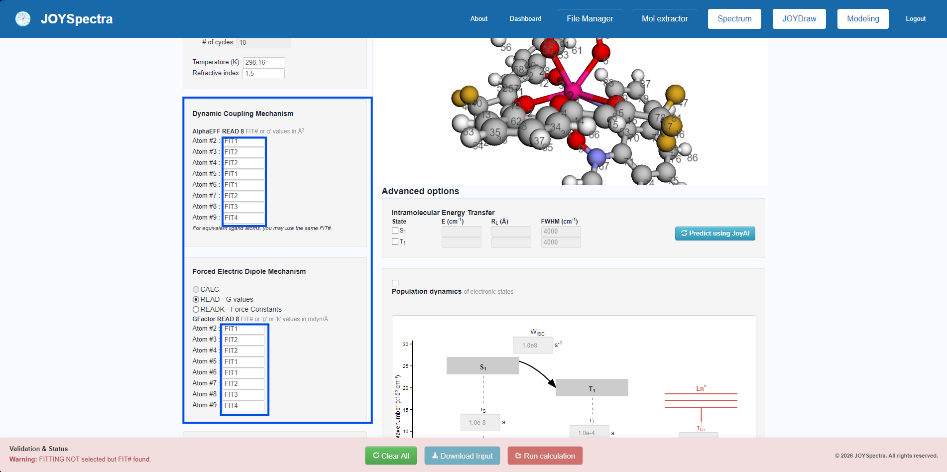
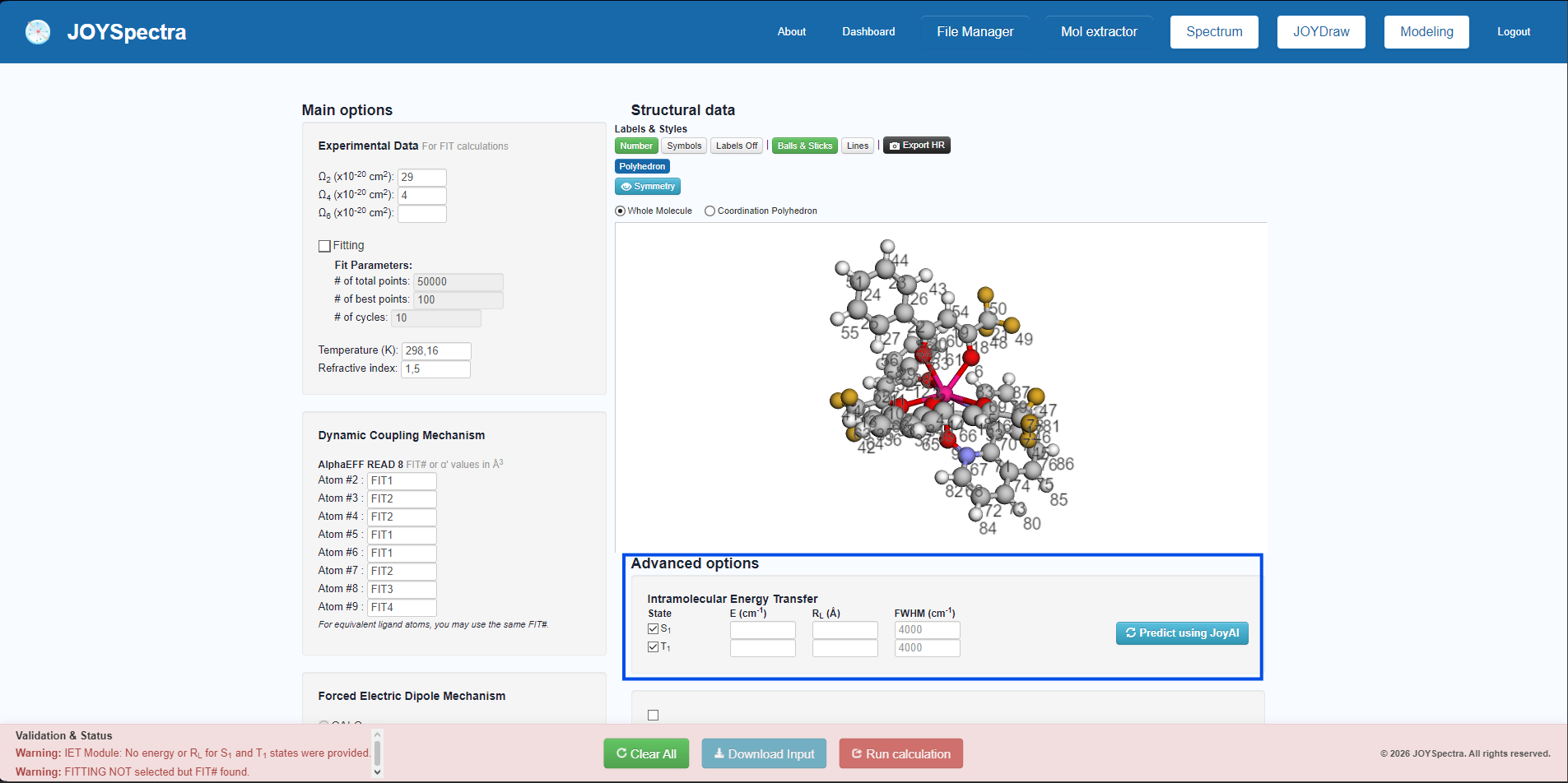
Step 4: In the "Advanced options" section, configure the intramolecular energy transfer parameters by filling in the energies E (cm-1) and distances RL (Å) for the S1 and T1 states, or click "Predict using JoyAI" to estimate the values automatically.
Step 5: In the "Separated Ligands (JoyAI)" window, verify and adjust the individual charges under "Total Charge" for each displayed organic ligand. After confirming the correct charges, click the "Run Pipeline" button to execute the prediction and generate the energy values.
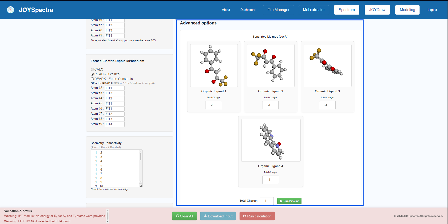
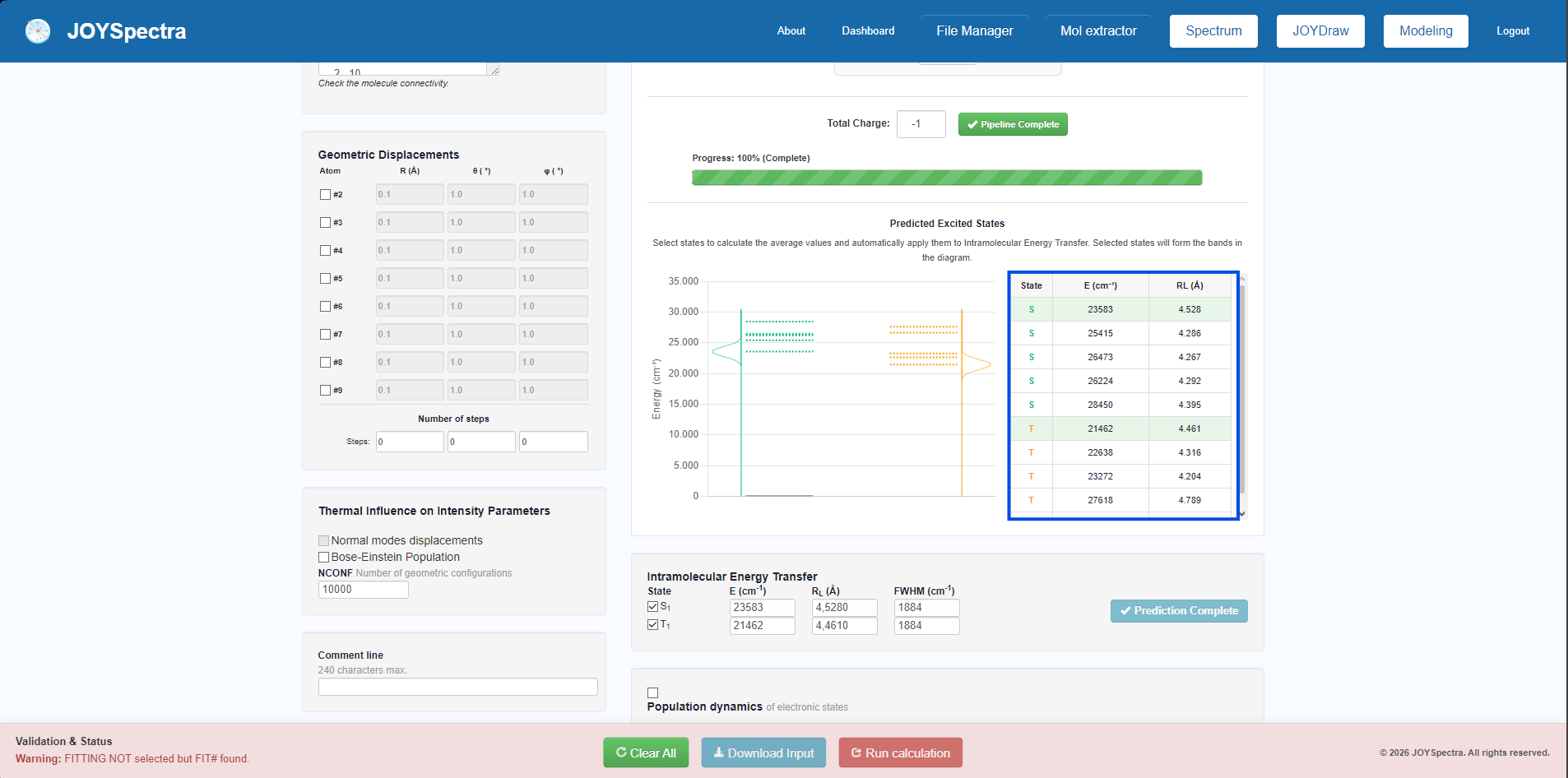
Step 6: After the prediction is complete, check the "Predicted Excited States" chart and table. Select the desired singlet (S) and triplet (T) states in the table so that the system calculates the average energy E (cm-1) and distance RL (Å) values, automatically populating them in the "Intramolecular Energy Transfer" panel.
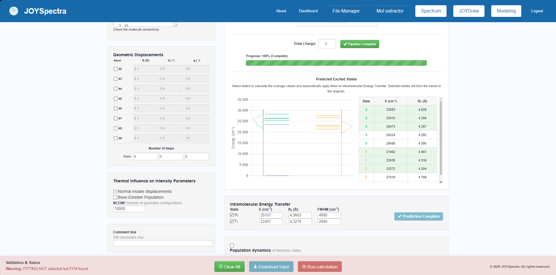
Step 7: In the "Predicted Excited States" table, you can select multiple states that you deem most appropriate for your system. By checking more than one level, the platform will automatically calculate the average of the energies and distances, updating the fields.
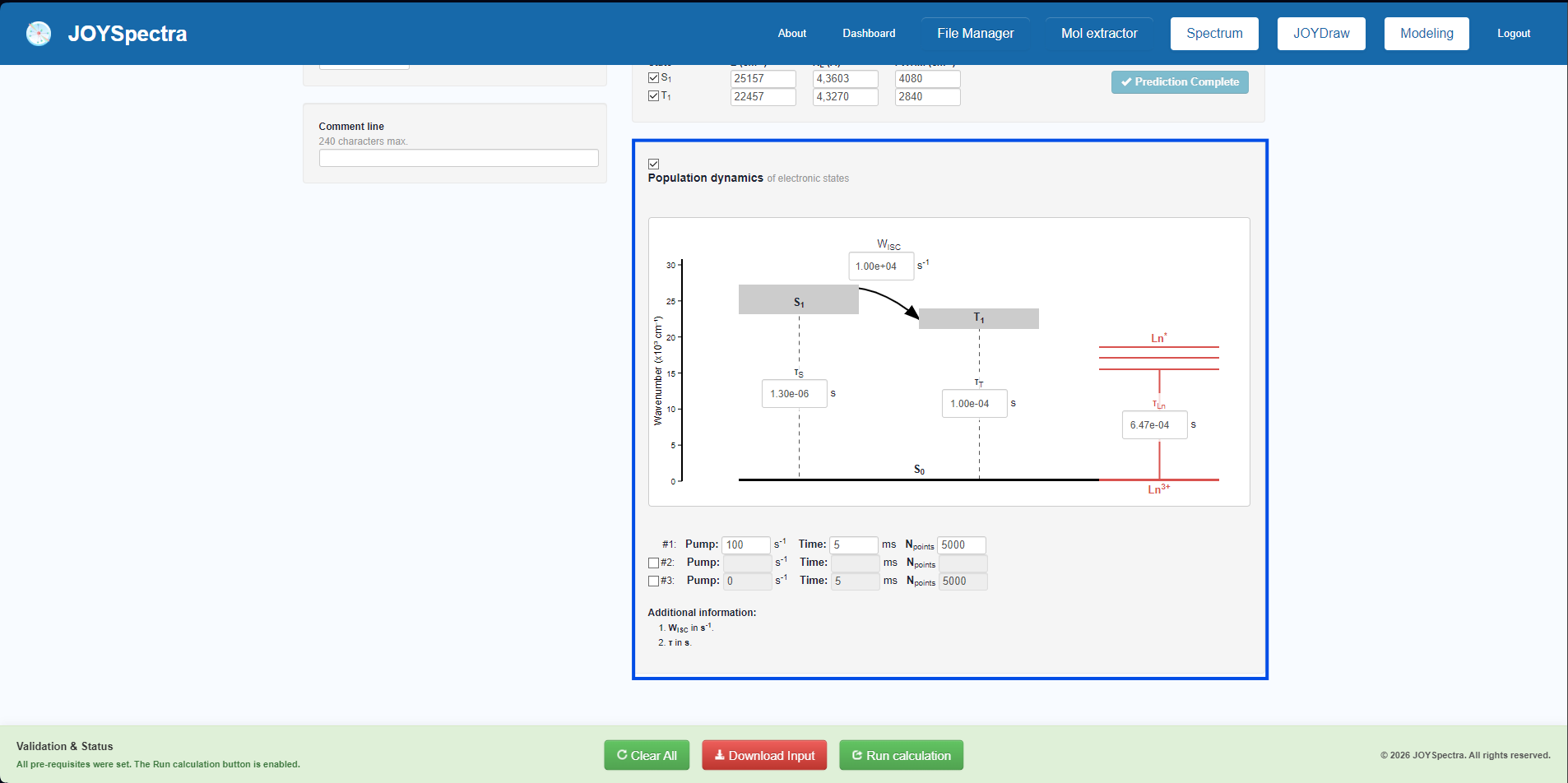
Step 8: Check the "Population dynamics" box to enable the calculation of the luminescence quantum yield and the population dynamics of the electronic states. Insert the experimental lifetime and transition rate parameters into the corresponding fields of the diagram.
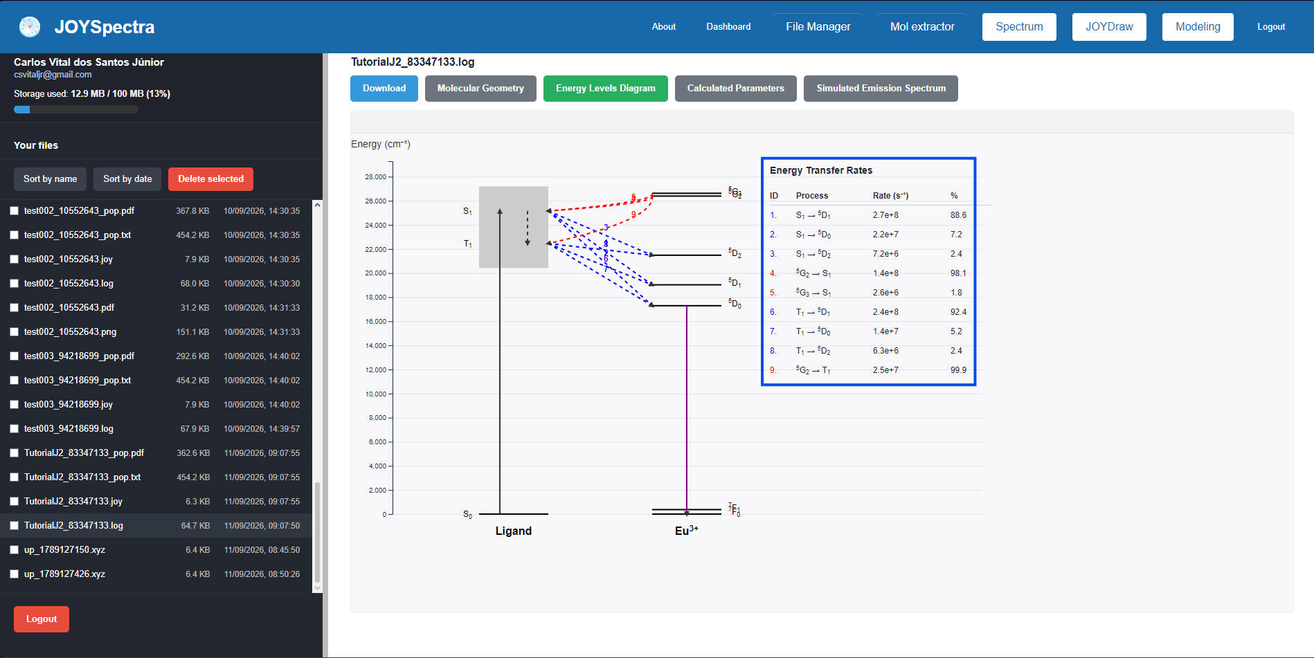
Step 9: In the File Manager, upon opening the final results file, access the "Energy Levels Diagram" tab to view the energy level diagram and the transfer rates table. Hover the mouse cursor over the rows in the table to highlight and inspect each transfer process individually.
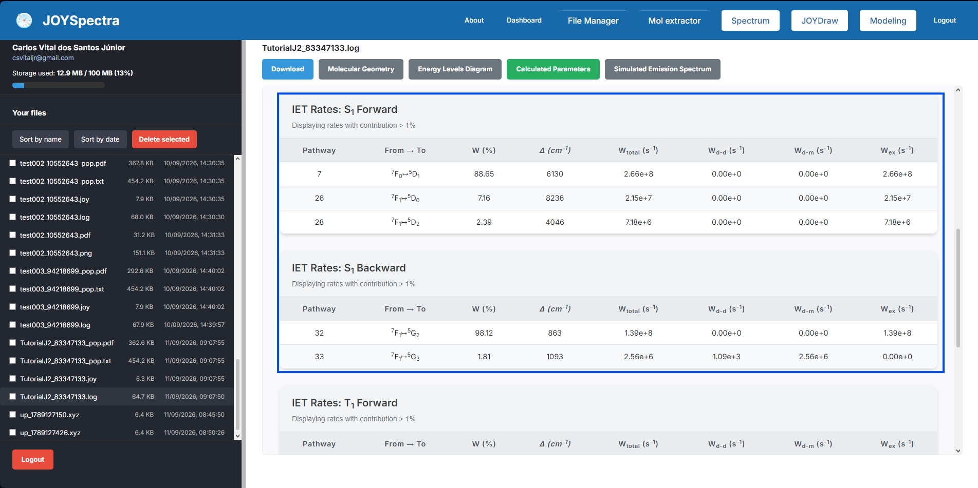
Step 10: In the File Manager, select the "Calculated Parameters" tab to view the calculated energy transfer parameters, such as the direct rates and back-transfer tables.

The ORCA software was used to perform single-point energy calculations using the GFN2-xTB method. For more details and advanced documentation, visit the Official ORCA Tutorials.
ORCA Program:
• Neese, F. Software update: the ORCA program system – Version 6.0 Wiley Interdiscip. Rev.: Comput. Mol. Sci., 2025, 15, 2, e70019 (DOI: 10.1002/wcms.70019).
• Neese, F. The ORCA program system Wiley Interdiscip. Rev.: Comput. Mol. Sci., 2012, 2, 1, 73–78 (DOI: 10.1002/wcms.81).
GFN-xTB Methods:
• Bannwarth, C.; Ehlert, S.; Grimme, S. GFN2-xTB—An Accurate and Broadly Parametrized Self-Consistent Tight-Binding Quantum Chemical Method... J. Chem. Theory Comput., 2019, 15 (3), 1652–1671 (DOI: 10.1021/acs.jctc.8b01176).
• Grimme, S.; Bannwarth, C.; Shushkov, P. A Robust and Accurate Tight-Binding Quantum Chemical Method... J. Chem. Theory Comput., 2017, 13 (5), 1989–2009 (DOI: 10.1021/acs.jctc.7b00118).
• Pracht, P.; Caldeweyher, E.; Ehlert, S.; Grimme, S. A Robust Non-Self-Consistent Tight-Binding Quantum Chemistry Method for Large Molecules. ChemRxiv, 2019 (DOI: 10.26434/chemrxiv.8326202.v1).